In this article I will try my best to explain what exactly a Lagrange Multiplier means and how these multipliers play important role in solving some of the crucial optimization problems in the context of machine learning.

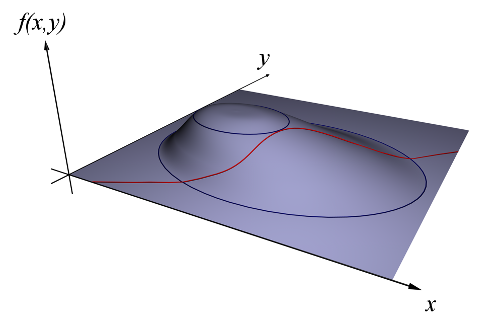
Before getting started with Lagrange multipliers lets understand contour lines. The better we understand contour lines, the more we can visualize whats happening with Lagrange multipliers.

A contour is a way to visualize a three-dimensional function in two dimensions. In such a representation of the function, for each point on a contour line, the function returns the same value. Lets consider the following three functions.

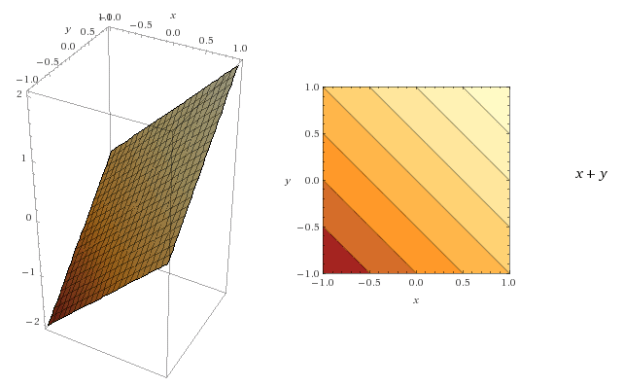
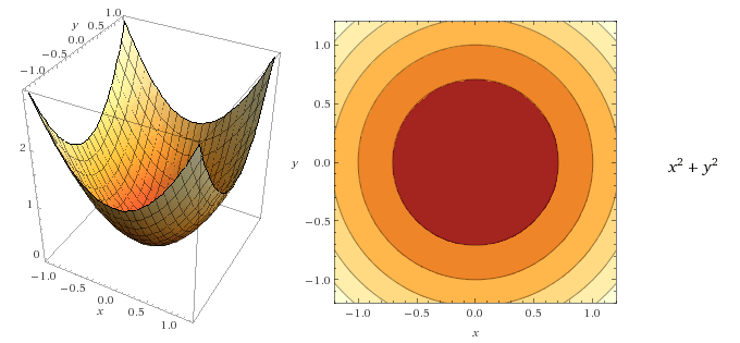
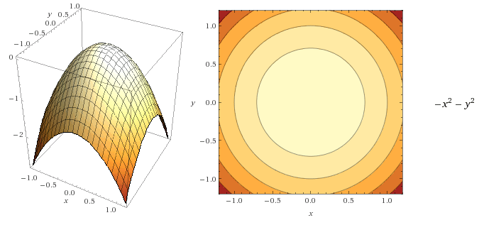
In all the above cases for each point on the contour line, the function returns the same value.

Now lets come back to our original discussion. Lets say we have an objective function f(x,y) which we need to maximize under a constraint of the form g(x,y)=c. Lets visualize this problem statement before we go deeper into our discussion.

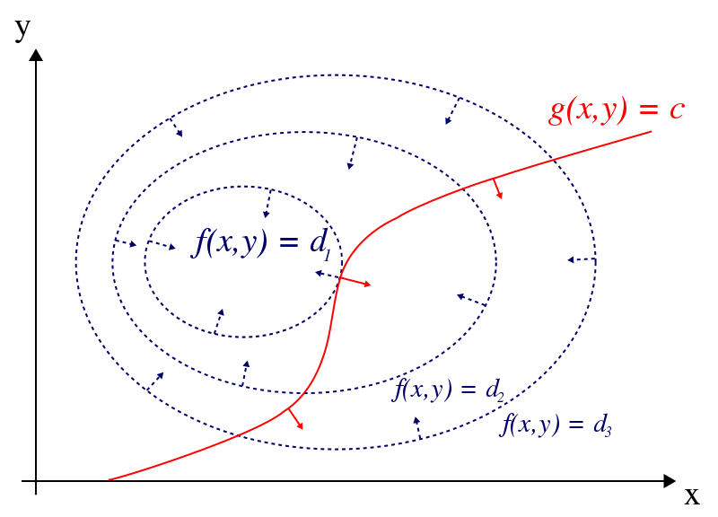
At any point (x,y), the gradient ∇f(x,y) is a vector which tells us the direction in which we should move inorder to increase f as efficiently as possible. As long as we are moving in that direction we are certainly going to increase f. This is the direction of steepest ascent. The gradient of any function evaluated at a particular point (x,y) always gives a vector perpendicular to the contour line passing through that point.

One thing we have to keep in mind that while climbing the hill we have to stay on the constraint curve g(x,y)=c all the time. In other words we are only allowed to move along the tangents to this constraint curve. Since these tangents are orthogonal to the gradient of the constraint function g, while moving along the constraint curve g(x,y)=c its value remain constant.

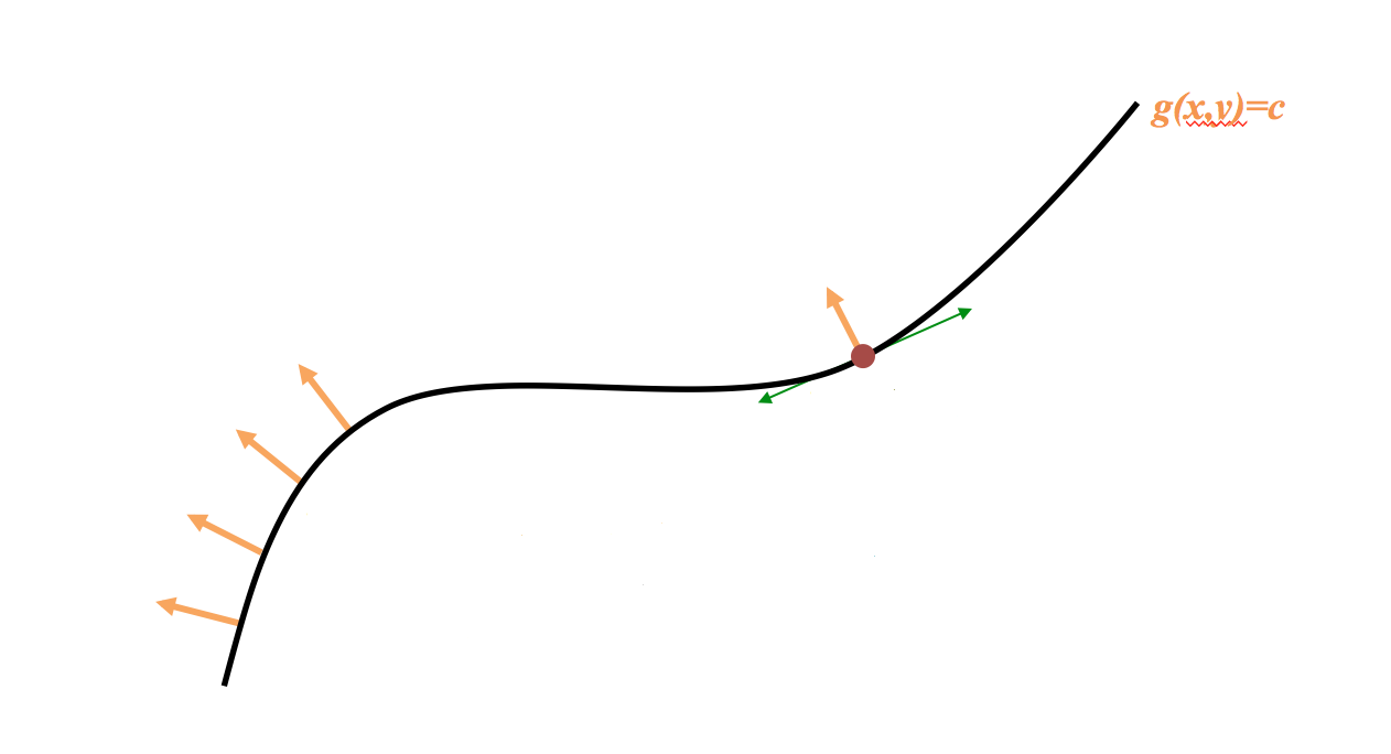
While moving along the constraint curve g(x,y)=c we need to simultaneously observe how we move on the surface of f. If we are moving in a direction that has a non-trivial component along the gradient ∇f(x,y), we are still going to increase f. The moment we can only move in a direction orthogonal to the gradient ∇f(x,y), then we won’t be able to increase f anymore. Here we have reached a local maximum. At this point the gradient of f and the gradient of g are pointing in the same direction. In other words, they are proportional. In other words, there is some constant λ such that the gradient of f is λ times the gradient of g. This λ is our Lagrange Multiplier.

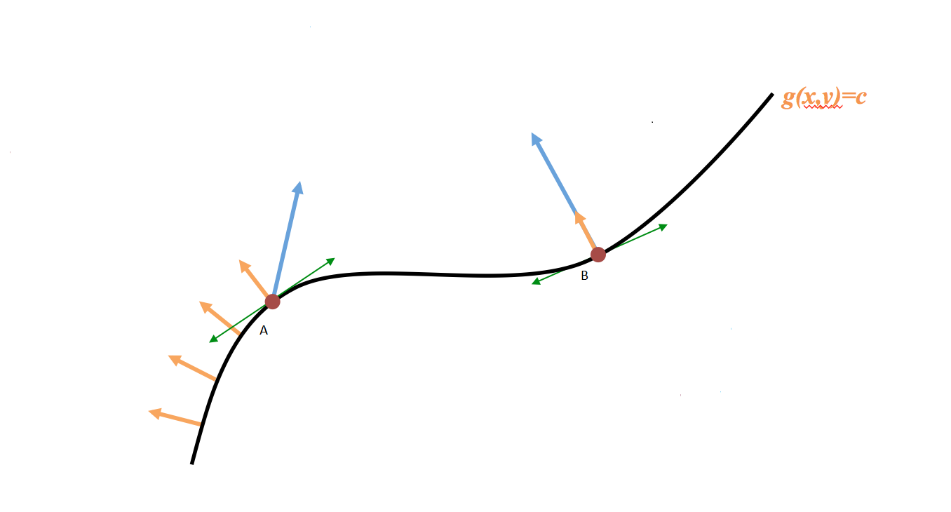
At point A the gradient of the function f to be maximized has a component along the direction we can move in. This is not the local maximum as we can increase f by moving to the right. At point B we can only move perpendicular to the gradient of f. Therefore this is the local maximum.

The final equation is ∇f(x,y)=λ∇g(x,y)

We can define a new function L as below:

L(x,y,λ)=f(x,y)-λ(g(x,y)-c)

We can call the function L as Lagrange function.

The final step is to set the gradient of L equal to the zero vector i.e, ∇L(x,y,λ)=0

So our objective is to find the critical points of L.

Lets solve a constraint optimization problem using Lagrange Multiplier Method.

Problem Statement :

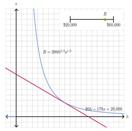
Suppose a factory produces some sort of widget that requires steel as a raw material. The human labor cost is $20 per hour for workers and the cost of steel is $170 per ton. Suppose the revenue is loosely modeled by the following equation :

f(h,s)= 200 x (h^2/3) x (s^1/3)

h represents hours of labor s represents tons of steel

If the total budget is $20000, then what is the maximum possible revenue ?

Solution

Per hour labor cost = $20 Per ton steel cost = $170

So the total cost of production = 20h + 170s , where h = total hours of labor and s = total tons of steel

As per as the problem statement 20h + 170s = 20000 ( This is our constraint since it is in the form g(h,s)=c , c=constant )

We need to maximize the objective function f(h,s) subject to the above constraint g(h,s).

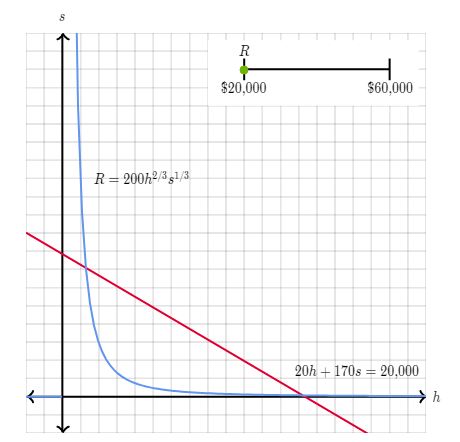
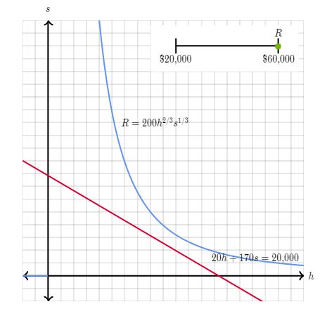
In the following diagrams , the objective function f(h,s) is represented as blue curve whereas the constraint g(h,s) is represented as red line. The values of f(h,s) yield a given revenue R which satisfies the constraint.

So we can write the Lagrange Function as below :

L(x,y,λ) = f(x,y)-λ(g(x,y)-c) = 200 x (h^2/3) x (s^1/3) - λ x (20h + 170s - 20000)

Next we set the gradient ∇L equal to the 0 vector. This is same as setting each partial derivative equal to 0.

First, we compute the partial derivative with respect to h.

∂L/∂h = 0
=> ∂ (200 x (h^2/3) x (s^1/3) - λ x (20h + 170s - 20000))/∂h = 0
=> 200 x (2/3) x (h^(-1/3)) x (s^(1/3)) - 20 x λ = 0 ………………..Equation I

Next, we compute the partial derivative with respect to s.

∂L/∂s = 0
=> ∂ (200 x (h^2/3) x (s^1/3) - λ x (20h + 170s - 20000))/∂s = 0
=> 200 x (1/3) x (h^(2/3)) x (s^(-2/3)) - 170 x λ = 0 ………………..Equation II

Finally we set the partial derivative with respective to λ equal to 0.

∂L/∂λ = 0
=> ∂ (200 x (h^2/3) x (s^1/3) - λ x (20h + 170s - 20000))/∂λ = 0
=> -20 x h -170 x s + 20000 = 0
20 x h + 170 x s = 20000 ………………..Equation III

The above equation is same as the constraint itself. So setting the partial derivative of L with respect to λ equal to 0 is same as re-writing the constraint.

Solving Equation I,II,III together we obtain
h ≈ 666.667
s ≈ 39.2157
λ ≈ 2.593

The maximum revenue can be computed as below

f(666.667,39.2157) = 200 x ((666.667)^2/3) x ((39.2157)^1/3) ≈ $51777